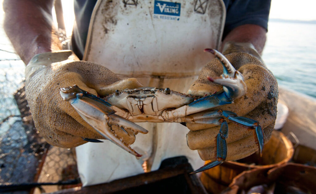
Last April, we met Captain CJ Canby at the Maryland Day / DC Climate Week and chatted about commercial crabbing in Chesapeake Bay and his concerns about changing water conditions in the areas where he works. That conversation led to a practical question: could water-quality instruments be incorporated into normal commercial crabbing operations and collect useful data over several days?
For researchers working in Chesapeake Bay, access is always part of the problem. Research vessels equipped with conventional instrumentation can collect excellent data, although vessel time, trained personnel, equipment and logistics make repeated measurements across a large area expensive. Commercial watermen, meanwhile, are already on the Bay throughout the season, repeatedly visiting the same fishing grounds and collectively covering a large area of water.
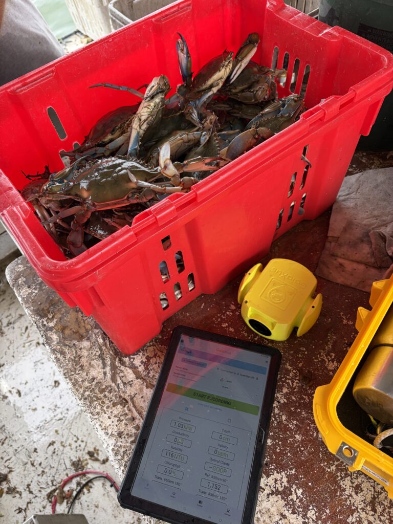
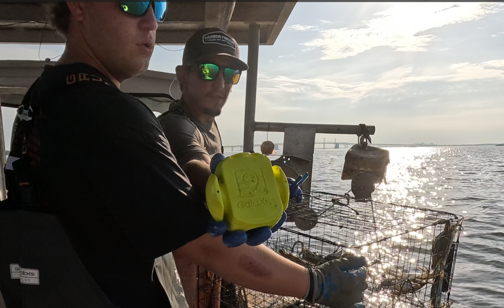
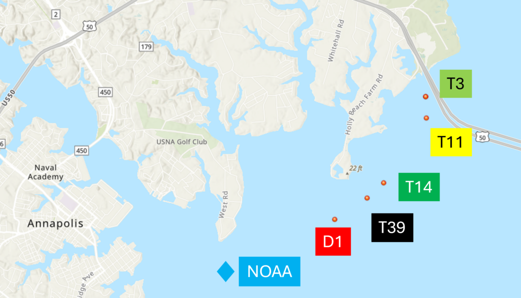
In June 2026, we worked with CJ aboard the F/V Miss Paula near Sandy Point State Park to test whether some of that existing activity could also support environmental monitoring. Five GaiaXus sensors were attached to commercial crab pots and left in the Bay for five days, from June 6 through June 11. The sensors collected measurements every 15 minutes, including temperature, salinity, turbidity, depth and chlorophyll-related optical data. After recovery, temperature, salinity and depth measurements were compared with available data from NOAA National Data Buoy Center Station 44063.
Monitoring as Part of Normal Operations
The first question was operational. If environmental monitoring interferes substantially with the work of the vessel, it is unlikely to become useful at scale.
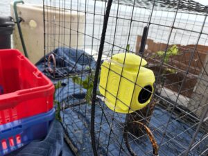
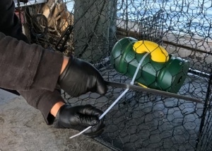
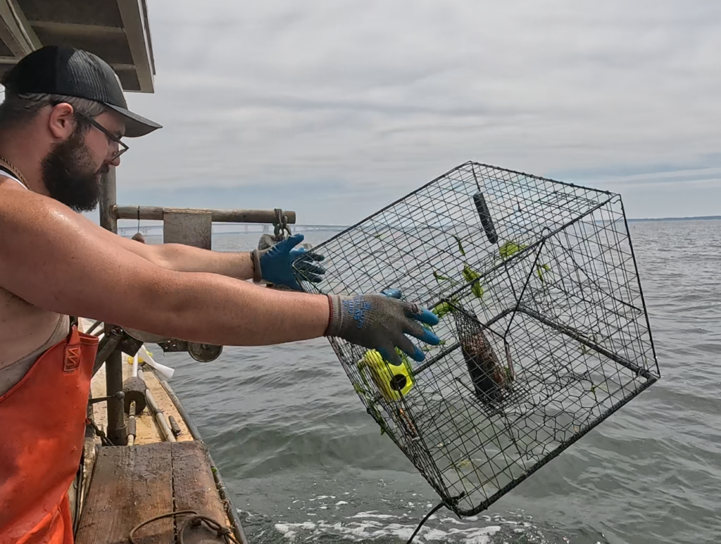
For this deployment, the sensors were attached directly to the crab pots with zip ties. Deployment and retrieval added less than 30 seconds to normal pot handling. After five days, the sensors were recovered relatively clean, with no visible damage or substantial algal contamination. Four of the five units still had battery capacity remaining.
The equipment was adapted to the way the waterman was already working. The crab pots provided the deployment platform, and the sensors went where the gear was already going. The same principle can apply to other environments. Around an oyster reef, for example, an instrument might be suspended from a buoy, mounted to a T-bar or attached to another existing structure. Distributed monitoring equipment therefore has to combine measurement quality with low cost, robustness and enough versatility to adapt to different field conditions.
Results
Deployment & Recovery
All sensors were deployed on different lines of pots, each experiencing slightly different underwater conditions at depths ranging from approximately 220 to 350 cm. The sensors were zip-tied into the pots and staged for deployment by the crew. Preparation of each sensor from the storage case to deployment readiness took approximately 30 seconds.
Upon retrieval, the sensors connected directly to the onboard mobile app and transmitted their data before they were removed from the pots. The crew removed the sensors while processing the catch and before the pots were cleaned in hot water. All sensors were relatively clean and showed no significant biofouling.
After cleaning, the sensors were returned to the laboratory, tested and recalibrated. Turbidity measurements remained within calibration, while the salinity sensors had drifted by approximately 10–15% and required recalibration.
Temperature
Temperature measurements from the five deployed sensors followed the same general temporal pattern as NOAA Station 44063 over the deployment period. The sensors also recorded repeated day-night variation in temperature.
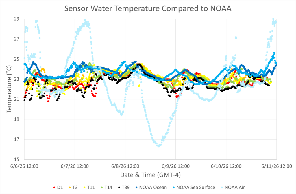
Figure 1. Temperature measurements from the five deployed sensors and NOAA Station 44063.
The data show diurnal oscillations that correspond broadly with the NOAA buoy data. NOAA also provides surface-water and atmospheric temperature measurements, which oscillate at greater amplitude, as expected, and in several cases appear to precede changes in the deeper water-temperature measurements.
Salinity
Salinity was derived from conductivity measurements, and all systems were calibrated before deployment.
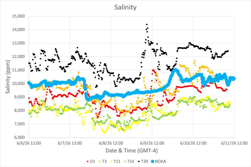
Figure 2. Salinity measurements from the five deployed sensors and NOAA Station 44063.
Salinity varied over time and among the five sensor locations. The instruments showed broadly similar temporal changes, with differences in absolute values among individual deployment sites. Of particular interest is the relatively sudden decrease recorded by all sensors after June 7, followed by a gradual increase over the next day.
While the NOAA buoy showed a relatively steady increase during this period, the five GaiaXus sensors recorded more pronounced oscillations in salinity. The changes were also not always synchronous among sensors. This is particularly noticeable shortly before June 9, when changes recorded by T39 occurred earlier and were more pronounced than those observed at the NOAA buoy or at the nearby D1 sensor.
Turbidity
The sensors were positioned approximately 25–30 cm above the seafloor, keeping the optical measurement channels above the sediment. All sensors were calibrated before deployment, and turbidity measurements were recorded in NTU. Comparable NOAA turbidity data were not available for this period.
Turbidity remained primarily between 0 and 40 NTU throughout the deployment. Temporary increases were evident across all sensors, although their magnitude varied among locations. Differences in bottom conditions and local currents may have influenced particle transport at each sensor location.
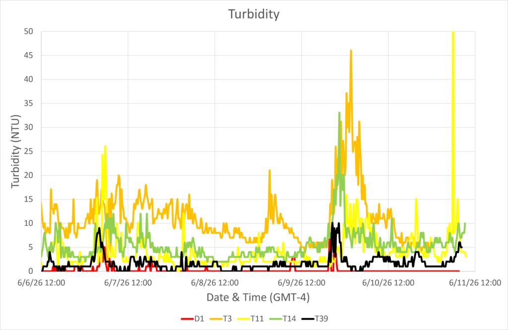
Figure 3. Relative turbidity measurements from the five deployed sensors.
The temporary changes in turbidity appeared to occur during the same periods as changes observed in depth and salinity. The GaiaXus probes contain both a nephelometric turbidity sensor, shown here, and a separate optical absorbance measurement system, which is not shown in this analysis.
Depth
Because the sensors remained at fixed locations near the seafloor, changes in measured depth primarily reflect changes in the height of the water column above them. Tidal variation is pronounced in this part of the Bay, and the approximately six-hour tidal cycle is clearly visible in all five sensor records as well as in the NOAA buoy data.
The sensors were deployed at different starting depths. GaiaXus sensors are rated to 10 m (approximately 30 ft), and the deepest deployment in this experiment was approximately 350 cm, well within the specified operating range.
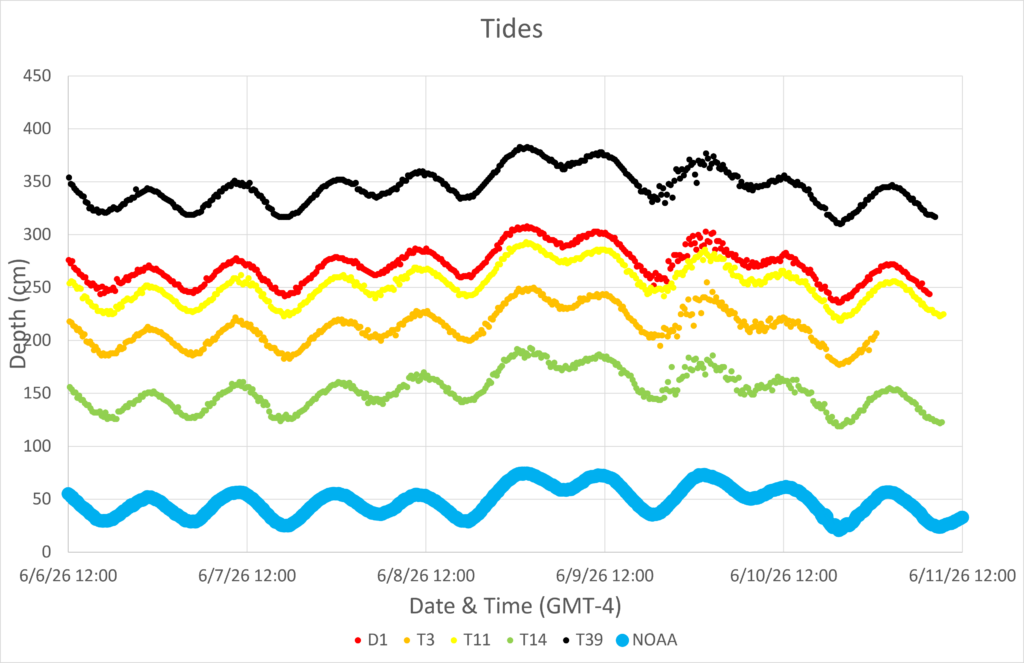
Figure 4. Depth measurements from the deployed sensors, showing the period associated with increased turbidity.
On June 10, all GaiaXus sensors recorded additional fluctuations superimposed on the normal tidal cycle. These fluctuations were not evident in the downstream NOAA buoy record. The observations therefore appear to represent a localized event and occurred during the same general period as changes in salinity and turbidity. The available data are not sufficient to determine the cause of these changes.
Discussion and Next Steps
Data
All sensors transmitted their data directly to the onboard mobile device when they were recovered. Cell phone coverage was good during this deployment, and the data were uploaded to GaiaXus cloud storage before the sensors had been removed from the crab pots. Research partners could therefore access the measurements within minutes of recovery.
Rapid access to the data makes it possible to review results while a deployment is still underway and adjust subsequent deployments if needed. It also allows onshore and offshore teams to work from the same dataset without waiting for instruments or data files to return from the field. Where internet access is unavailable, the data remain stored on the mobile device and are transmitted once a connection becomes available, allowing the same workflow to be used in remote locations.
Each measurement is associated with a time index and GPS location. The platform transfers the data through an API to ESRI ArcGIS, where measurements can be mapped immediately after retrieval and downloaded for further analysis. This combination of automated transfer, georeferencing and rapid access becomes increasingly important as the number of instruments and deployment locations increases. For larger projects, it also provides a practical way for geographically distributed research teams to work with the same dataset soon after it is collected.
Sensor Performance
The sensors were deployed and recovered during normal commercial fishing operations without interfering with the work of the vessel. Attachment to the crab pots was simple, and the five-day deployment did not require a separate sampling procedure or specialized handling by the crew.
After recovery, there was very little visible fouling on either the exterior surfaces or inside the optical measurement channel. Fouling remains an important consideration for longer deployments because accumulation of algae, sediment or other material can affect optical measurements and eventually reduce data quality. The internal optical chamber is made from borosilicate glass, which provides a relatively resistant surface, although no exposed optical system is completely immune to fouling under field conditions.
The five-day deployment therefore provides an initial indication that the sensors are suitable for this type of use, while longer deployments are needed to establish the practical limits. Deployments of approximately two weeks under different depths, currents, temperatures and biological conditions would provide a better assessment of fouling, sensor stability and maintenance requirements. After this deployment, the instruments were cleaned with warm water, soap and stiff brushes and prepared for use at another site.
The physical configuration is also important for distributed monitoring. In this study, the sensors were attached directly to crab pots, although the same instrument could be suspended from a buoy, mounted to a T-bar or attached to another fixed structure. A distributed monitoring system has to combine measurement performance with enough robustness and flexibility to adapt to the environment in which the measurements are being collected.
Data Consistency
The GaiaXus sensors showed temporal patterns that were broadly consistent with measurements from the nearby NOAA monitoring station. This comparison does not constitute a formal validation of the instruments, although it provides a useful external reference for determining whether the sensors were capturing the larger environmental changes occurring during the deployment.
The instruments were programmed to record one measurement every 15 minutes. This interval was sufficient to identify changes in temperature, salinity, turbidity and depth over the five-day period while keeping the total data volume small. The localized changes observed in depth, salinity and turbidity also showed that the sampling interval was sufficient to detect relatively short-term events.
In retrospect, a five-minute sampling interval would have provided greater temporal resolution during these periods and may have allowed the timing and sequence of the observed changes to be defined more precisely. Increasing the sampling frequency from 15 minutes to five minutes would have tripled the number of measurements, although the resulting dataset would still have been easily manageable.
Sampling frequency can therefore be adjusted to the scientific question without substantially changing the field procedure. Longer deployments may favor lower sampling frequencies, while experiments focused on short-term events can collect measurements more frequently. As larger numbers of sensors are deployed, this flexibility allows spatial coverage, temporal resolution and deployment duration to be balanced for the particular monitoring objective.
From Five Sensors to a Distributed Monitoring Network
The five sensors in this deployment covered a relatively small area for five days, yet they demonstrated the basic elements required for distributed monitoring: multiple instruments operating simultaneously at different locations, repeated measurements over time, and automated aggregation of the resulting data. Measurements from an individual sensor describe conditions at one location, while the combined dataset begins to describe how those conditions vary across an area.
Commercial watermen provide an unusual opportunity to extend this model. Their vessels already operate regularly across large parts of Chesapeake Bay, often returning to the same fishing grounds and gear locations throughout the season. Incorporating sensors into those existing operations could give researchers repeated access to locations that would otherwise require dedicated vessel time, personnel and equipment. The objective is to complement research cruises and established monitoring stations by increasing the density of observations between them.
The potential increases substantially as the number of instruments grows. A network of 100 or 300 sensors deployed through commercial fishing operations could collect measurements from hundreds of locations at comparable time intervals. Individual datasets could then be combined to examine environmental conditions over larger areas while retaining the spatial and temporal resolution of the original measurements. Achieving similar coverage with dedicated research vessels and conventional instrumentation would require a very different level of resources.
This type of network could also address questions that are difficult to study using either a fixed station or an occasional sampling cruise. Temperature, salinity, turbidity and other bottom-water conditions can vary over relatively short distances and periods of time. These conditions are relevant to crab habitat and commercial yield, although the present study was not designed to establish a relationship between the environmental changes we observed and crab catch. A sufficiently dense monitoring network could provide the environmental context needed to begin examining such relationships systematically.
The June deployment demonstrated that the practical components of this approach can work within normal commercial fishing operations. The sensors remained deployed for several days, collected continuous measurements and were recovered with little disruption to the crew. Scaling the approach will require additional work on sensor performance, deployment duration, data quality and network design. Combining robust, low-cost instrumentation with the routine activity of commercial watermen could provide water-quality data at a spatial and temporal resolution that is difficult to achieve with conventional monitoring alone.